Player Consistency Modeling

A league-wide survey

In our last post, we detailed our negative binomial stat prediction model. This model learns a value for how consistent each player is. Here, we’ll look across the league at various stats, and see who is consistent and who isn’t.

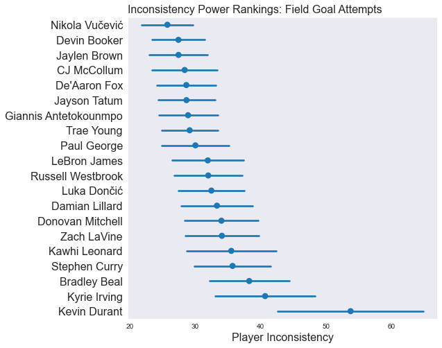
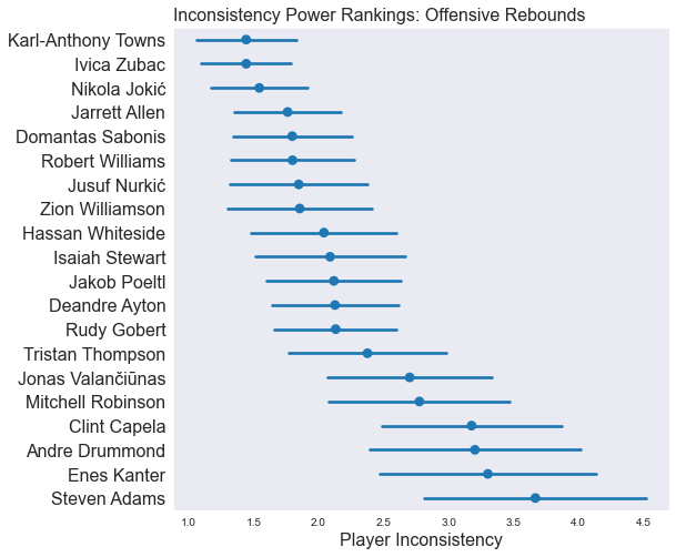
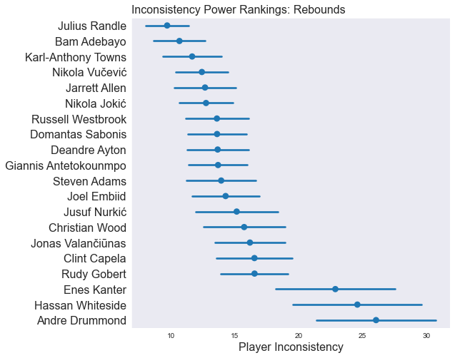
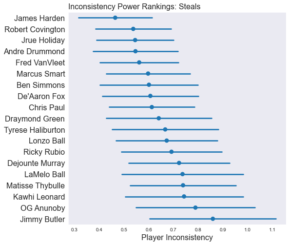
In the following plots, we’re showing how inconsistent our model thinks a handful of players are for each stat. Players at the top of the plot are consistent game-to-game, and players at the bottom of the plot are less consistent (more fun to watch). Importantly, the confidence intervals show how certain the model is about it’s value for the players’ inconsistency.

We’ll give some general notes at the bottom, but there’s a lot to unpack here.

As we said previously: although the value in the plots has a real-life meaning related to how much variance each player is predicted to have game-to-game, it’s easiest just to think of this as Inconsistency Power Rankings.

The stat-of-interest is in the title, starting with points:

Some general notes:

• We included the “Steals” plot to make a point. Sometimes, you can’t draw any conclusions from a model. Look at the uncertainty in those values. You really can’t make any conclusive statements about how consistent players are in getting steals.

• In contrast to steals, you can make a pretty strong statement about Kevin Durant’s inconsistency in FGA.

• Some players are consistently consistent. Karl-Anthony Towns is basically the most consistent player at getting to the free throw line, rebounding, and scoring.

• As players get more inconsistent, the model has a harder time understanding precisely how inconsistent they are.

Looking Ahead

I’m going biking for a week or so in Utah. If anyone has recommendations, please let me know.

Model

For details about the model, see the previous post. It’s a hierarchical negative binomial regression.

data {
   
    int<lower=0> n_players;
    int<lower=0> n_stats;
    int stats[n_stats];
    int stats_player_index[n_stats];

}

parameters {

    // Mu terms
    vector<lower=0>[n_players] player_value;

    // Hierarchical Parameters
    real<lower=0> theta_bar;
    real<lower=0> sigma_bar;

    // Variance Terms
    vector<lower=0>[n_players] overdispersion;

}


model {

    // Hierarchical Prior on mu
    theta_bar ~ normal(0, 25);
    sigma_bar ~ cauchy(0, 5);
    player_value ~ normal(theta_bar, sigma_bar);

    //  Prior on Variance
    overdispersion ~ gamma(2, 2);


    // Negative Binomial Regression

    for (stat in 1:n_stats) {
      stats[stat] ~ neg_binomial_2(player_value[stats_player_index[stat]], overdispersion[stats_player_index[stat]]);
  }
}

generated quantities {
   int player_36_estimate[n_players];

   vector[n_players] player_variance;

   for (player in 1:n_players) {
     player_36_estimate[player] = neg_binomial_2_rng(player_value[player], overdispersion[player]);

     player_variance[player] = player_value[player] * player_value[player] / overdispersion[player];
   }

}