Predicting NBA Scores Part 2

Improving our model's priors

In our last post, we gave a brief overview of our score-line prediction model. There is a glaring list of improvements to make. In this post (and the following post), we’ll focus on prior modeling. Specifically, we’ll look at the prior on home field advantage as an illustration.

As always, our full model is at the bottom of this post.

Home Field Advantage

Our original model had a home field advantage parameter baked into it. Here is what the posterior of that parameter looked like:

Home field advantage estimates from our original score-line prediction model

Home field advantage is somewhere between 2 and 2.5 points this season. But there is a lot of variance in that estimate. Home field advantage might be as low as half a point or as high as 4 points.

But what prior did we put on that parameter?

// Home field advantage, about 2 points
home_field_advantage ~ normal(2, 2);

I thought: “eh, home field advantage is about two points, and if I put a large variance on it, I should be safe.” But what is that prior actually saying? Here’s what that prior distribution looks like:

Home field advantage from our original model. normal(2, 2)

There’s one glaring problem: do we really expect home court advantage to be negative? This prior gives a 15% probability that home field advantage is less than zero. There’s also a slightly less glaring problem: Do we really expect home field advantage to be greater than 5 points? This prior gives a 7% probability that home field advantage is greater than 5 points.

Let’s develop a prior that more closely aligns with our domain expertise. The easiest (and arguably best) way to develop a prior isn’t to ask: what values do we expect our parameter to be. Instead, ask: what values do we not expect our parameter to be? This amounts to finding two thresholds: an upper bound and a lower bound (we don’t expect our parameter value to fall outside of those thresholds). How do we determine those thresholds? I like the mindset from this post on prior modeling: “Once we've transitioned from "I mean it's possible" to "oh, no, that's ridiculous" we know we've passed a meaningful threshold”.

To me, the lower bound on the number of points home field advantage is worth before it becomes ridiculous is zero. I can buy there is no home court advantage, but I’m not ready to buy that it’s negative. The upper bound? I think anything above 5 points would be ridiculous.

To convert those thresholds into a prior model, we do two things:

1. For the lower threshold (0 points), we use a hard threshold. We’ll sample from a half-normal(0, sigma) to prevent negative values.

2. For the upper threshold (5 points), we’ll use a soft threshold. We’ll adjust the sigma in our half-normal(0, sigma) such that 99% of the prior density falls between 0 and 5 points. This doesn’t completely prevent home field advantage from being greater than 5, but it aligns with our expectation that it would be very unlikely.

This is our refined prior distribution:

Our refined home field advantage prior: half-normal(0, 1.95).

I chose 5 points as the upper threshold for home field advantage. But what happens if you disagree? Below, I’m plotting the resulting home field advantage posterior distributions. You can that see if you think home court advantage is way more (20 points for illustration), it doesn’t really affect the posterior probability. If you think the threshold is lower (2 points for illustration) then it really affects our final model.

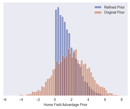
Comparing our refined prior to our original prior

This is our original prior compared to our refined prior. It’s nice to see no values below zero and unreasonably large values less likely.

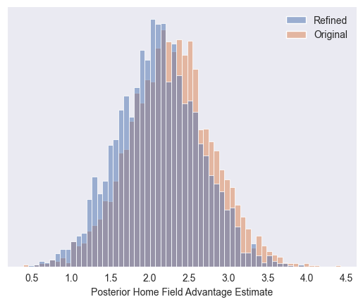
How did our prior refinement affect our resulting posterior estimate of home field advantage? Not much. The extreme values are suppressed a bit, in favor of more mild values.

Model Predictions

As before, our model is pumping out score line predictions (with a now-principled, albeit basically unchanged, home field advantage estimate).

Looking ahead

We have all sorts of wonky priors. The other ones are trickier to model in a principled manner, but we’ll work through it.

Stan Model

// Heirarchical IRT regression
//
// This models the points of home and away teams
// as a function of the latent offensive and defensive 
// strength of the teams.
//
// Specifically, this version tries to improve on the
// prior modeling.

data {
    // Number of games
    int<lower=1> N_games;

    // Number of teams in the league
    int<lower=1> N_teams;

    // Home and away points scored in each game
    array[N_games] int<lower=0> home_points;
    array[N_games] int<lower=0> away_points;

    // Team index for each game
    array[N_games] int<lower=1, upper=N_teams> home_team;
    array[N_games] int<lower=1, upper=N_teams> away_team;

    // Threshold for home field advantage
    // 99% of the density should be between 0 and this value
    real home_field_advantage_threshold;
}

transformed data {
    // Section 3.3.1 https://betanalpha.github.io/assets/case_studies/prior_modeling.html
    real home_field_advantage_prior_sigma = home_field_advantage_threshold / 2.57;
}

parameters {
    // Latent offensive and defensive strength of each team
    // Hierarchical prior
    vector[N_teams] theta_offense;
    vector[N_teams] theta_defense;
    real theta_offense_bar;
    real theta_defense_bar;
    real<lower=0> sigma_offense_bar;
    real<lower=0> sigma_defense_bar;

    // Noise in the points (same for home and away teams)
    real<lower=0> sigma_points;

    // Home field advantage is extremely unlikely to be negative
    real <lower=0> home_field_advantage;
}

model {

    // Prior Modeling

    // Average strength of the teams
    theta_offense_bar ~ normal(116, 10);

    // Home field advantage
    // Put 99% of dennsity between 0 and input {home_field_advantage_threshold}
    home_field_advantage ~ normal(0, home_field_advantage_prior_sigma);

    // Variations of the teams strength
    sigma_offense_bar ~ cauchy(0, 5);
    sigma_defense_bar ~ cauchy(0, 5);

    // Individual team strength
    theta_offense ~ normal(theta_offense_bar, sigma_offense_bar);
    theta_defense ~ normal(0, sigma_defense_bar);

    // Gaussian noise in the points
    sigma_points ~ cauchy(0, 5);

    // Likelihood
    for(game in 1:N_games) {
        // Team points modeled as gaussian
        real home_points_regression = home_field_advantage + theta_offense[home_team[game]] + theta_defense[away_team[game]];
        real away_points_regression = theta_offense[away_team[game]] + theta_defense[home_team[game]];
        home_points[game] ~ normal(home_points_regression, sigma_points);
        away_points[game] ~ normal(away_points_regression, sigma_points);    
    }
}

generated quantities {

    // Remove the mean from the latent variables
    vector[N_teams] theta_defense_centered;

    for (i in 1:N_teams) {
        theta_defense_centered[i] = theta_defense[i] - mean(theta_defense);
    }

    vector[N_teams] theta_offense_centered;

    for (i in 1:N_teams) {
        theta_offense_centered[i] = theta_offense[i] - mean(theta_offense);
    }
}